First, I’ll create a ‘dummy’ dataset that we can use to explore the CCA technique.
Show code
# clean environmentrm(list =ls())# Load necessary librarylibrary(MASS) # For generating correlated data# Create a synthetic datasetcreate_dataset <-function(n =100, means, Sigma) { data <- MASS::mvrnorm(n = n, mu = means, Sigma = Sigma)colnames(data) <-c("DrivingAccuracy", "PuttingAccuracy", "AverageScore", "EaglesPerRound", "WindSpeed", "Rainfall", "Temperature", "CourseDifficulty")return(as.data.frame(data))}# Define means and a covariance matrix for the variablesmeans <-c(60, 50, 72, 0.5, 10, 5, 70, 7)Sigma <-matrix(c(1, 0.2, 0, 0, -0.6, -0.7, 0, -0.1,0.2, 1, 0, 0, 0, 0, 0, 0,0, 0, 1, 0, 0, 0, 0, -0.5,0, 0, 0, 1, 0, 0, 0, 0,-0.6, 0, 0, 0, 1, 0, 0, 0,-0.7, 0, 0, 0, 0, 1, 0, 0,0, 0, 0, 0, 0, 0, 1, 0,-0.1, 0, -0.5, 0, 0, 0, 0, 1), ncol =8)# Generate the datasetset.seed(123) # For reproducibilitygolf_dataset <-create_dataset(n =100, means, Sigma)# Round all columns in the dataframe to 2 decimal placesgolf_dataset <-data.frame(lapply(golf_dataset, function(x) {if(is.numeric(x)) round(x, 2) else x}))rm(Sigma)
Step Two: Examine the correlations
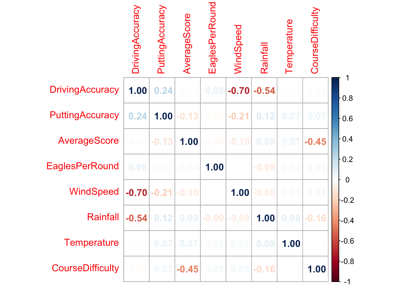
Remember that CCA is about the correlations that exist between the variables in our two sets of variables. Before digging too deep, it’s helpful to explore where those underlying correlations might exist.
# Load packageslibrary(ggplot2)library(corrplot)
corrplot 0.92 loaded
cor_matrix <-cor(golf_dataset) # create the correlation matrixcov_matrix <-cov(golf_dataset) # create the covariance matrix# Visualise correlation matrixcorrplot(cor_matrix, method ="number")
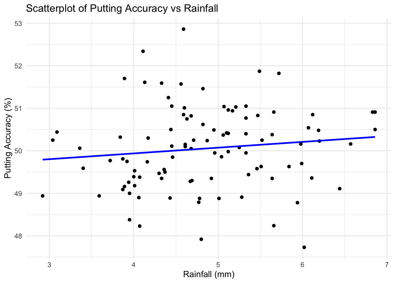
# more visualisations of the variables# Example 1# Scatterplot for Putting Accuracy vs Rainfallggplot(golf_dataset, aes(x = Rainfall, y = PuttingAccuracy)) +geom_point() +geom_smooth(method ="lm", color ="blue", se =FALSE) +labs(title ="Scatterplot of Putting Accuracy vs Rainfall",x ="Rainfall (mm)",y ="Putting Accuracy (%)") +theme_minimal()
`geom_smooth()` using formula = 'y ~ x'
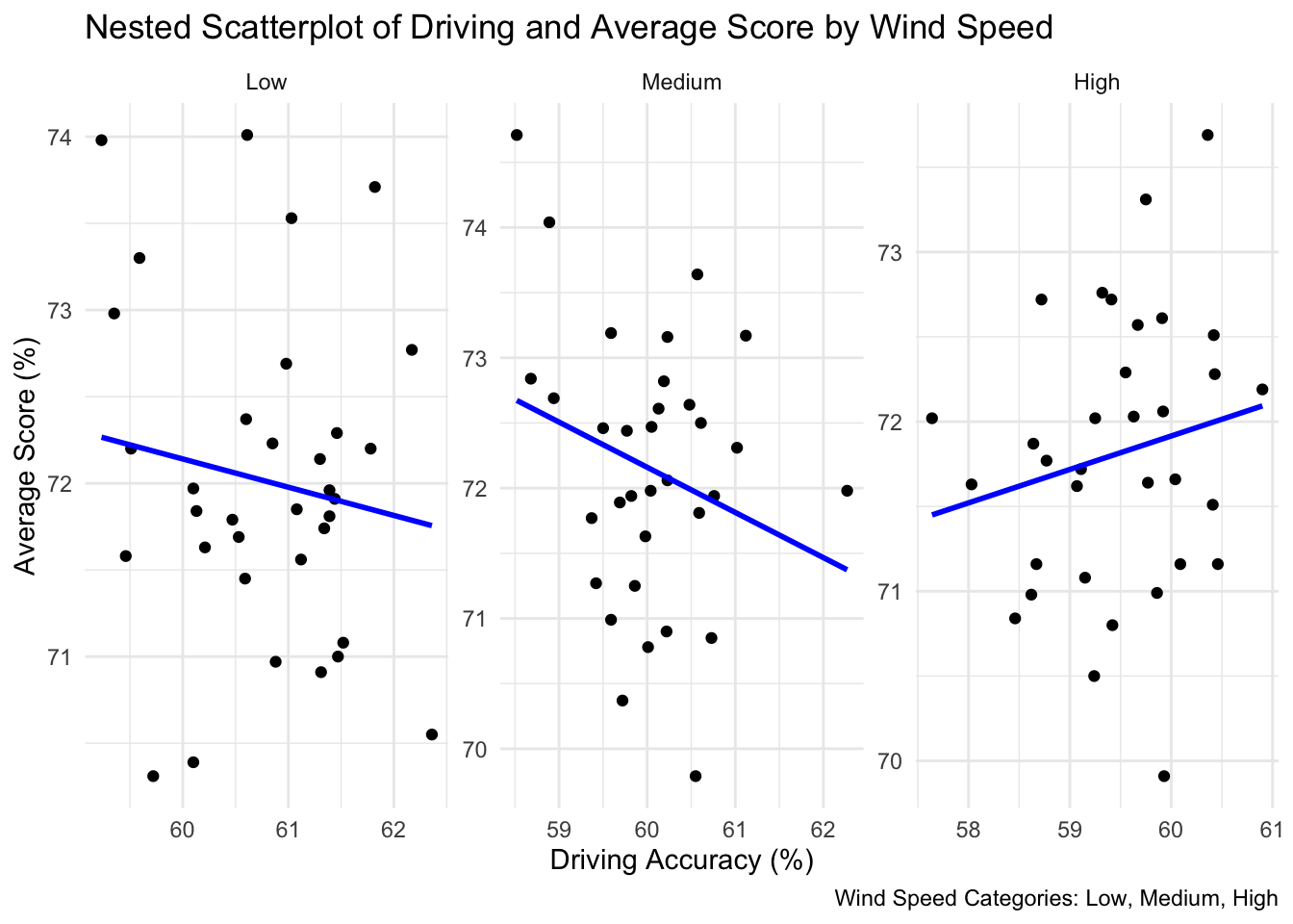
## Example 2# Categorise Wind Speed into 'Low', 'Medium', and 'High'golf_dataset$WindSpeedCategory <-cut(golf_dataset$WindSpeed, breaks =quantile(golf_dataset$WindSpeed, probs =0:3/3),labels =c("Low", "Medium", "High"), include.lowest =TRUE)# Nested Scatterplotggplot(golf_dataset, aes(x = DrivingAccuracy, y = AverageScore)) +geom_point() +geom_smooth(method ="lm", color ="blue", se =FALSE) +facet_wrap(~ WindSpeedCategory, scales ="free") +labs(title ="Nested Scatterplot of Driving and Average Score by Wind Speed",x ="Driving Accuracy (%)",y ="Average Score (%)",caption ="Wind Speed Categories: Low, Medium, High") +theme_minimal()
I must split the dataset into two parts; one contains the performance-related variables, and one contains the condition-related variables. Remember, we’re trying to explore how these two sets are associated.
Most importantly, I can display the canonical correlations. these tell me the overall associations between the two sets of variables. The higher the number in relative terms, the stronger the relationship.
We will have the same number of canonical correlations as the smallest number of variables in either set.
cc1 <-cc(performance, conditions) # display the canonical correlationscc1$cor
[1] 0.94379531 0.45876017 0.25324247 0.05955601
Step Seven: Display Raw Canonical Coefficients
These help us explore the association between the sets further. They tells us strongly each variable contributed to each of the relationships represented by our canonical correlation.
A similar concept can be found in canonical loading, which are the correlations between the variables and the canonical variates. Remember, these variates are a type of latent variable.
Finally, we can test what we’ve found. We look to see the significance of each of the canonical dimensions identified earlier and, if p < 0.05, we can say that there is a significant association overall between the two sets of variables.
# tests of canonical dimensionsrho <- cc1$cor## Define number of observations, number of variables in first set, and number of variables in the second set.n <-dim(conditions)[1]p <-length(conditions)q <-length(performance)## Calculate p-values using the F-approximations of different test statistics:p.asym(rho, n, p, q, tstat ="Wilks")
Wilks' Lambda, using F-approximation (Rao's F):
              stat     approx df1      df2      p.value
1 to 4:  0.0804393 22.5671350  16 281.7023 0.0000000000
2 to 4:  0.7362838  3.3732631   9 226.4882 0.0006674902
3 to 4:  0.9325488  1.6700815   4 188.0000 0.1586524218
4 to 4:  0.9964531  0.3381567   1  95.0000 0.5622724374
Now I’ll do the same but using standardised conditions:
First, run the following code in RStudio which will create a synthetic dataset called health_dataset.
rm(list =ls())# Load necessary librarylibrary(MASS) # For generating correlated data# Function to create a synthetic datasetcreate_dataset <-function(n =100, means, Sigma) { data <- MASS::mvrnorm(n = n, mu = means, Sigma = Sigma)colnames(data) <-c("CalorieIntake", "ProteinContent", "VitaminLevels", "WaterIntake","StressLevel", "MoodRating", "SleepQuality", "ConcentrationLevel")return(as.data.frame(data))}# Define means and a covariance matrix for the variables# These are example values and can be adjustedmeans <-c(2000, 50, 100, 2, 5, 7, 7, 7) # Example mean values for each variableSigma <-matrix(c(1, 0.5, 0, 0, 0, 0.3, 0.3, 0,0.5, 1, 0, 0, 0, 0.2, 0.4, 0,0, 0, 1, 0, -0.2, 0.2, 0, 0,0, 0, 0, 1, -0.3, 0.1, 0.2, 0.1,0, 0, -0.2, -0.3, 1, -0.4, -0.5, -0.3,0.3, 0.2, 0.2, 0.1, -0.4, 1, 0.6, 0.4,0.3, 0.4, 0, 0.2, -0.5, 0.6, 1, 0.5,0, 0, 0, 0.1, -0.3, 0.4, 0.5, 1), ncol =8)# Generate the datasetset.seed(123) # For reproducibilityhealth_dataset <-create_dataset(n =500, means, Sigma)# Calculate correlation and covariance matrixcor_matrix <-cor(health_dataset) # create the correlation matrixcov_matrix <-cov(health_dataset) # create the covariance matrix
Now, examine the correlations between the variables. Use any of the techniques you have previously learned about.
# Load packageslibrary(ggplot2)library(corrplot)cor_matrix <-cor(health_dataset) # create the correlation matrixcov_matrix <-cov(health_dataset) # create the covariance matrix# Visualise correlation matrixcorrplot(cor_matrix, method ="number")
# more visualisations of the variables# Example 1# Scatterplot of Calorie Intake and Sleep Qualityggplot(health_dataset, aes(x = CalorieIntake, y = SleepQuality)) +geom_point() +geom_smooth(method ="lm", color ="blue", se =FALSE) +labs(title ="Scatterplot of Calorie Intake and Sleep Quality",x ="Intake (cals)",y ="Sleep Quality (low - high)") +theme_bw()
## Example 2# Categorise Mood Rating into 'Low', 'Medium', and 'High'health_dataset$MoodRatingCat <-cut(health_dataset$MoodRating, breaks =quantile(health_dataset$MoodRating, probs =0:3/3),labels =c("Low", "Medium", "High"), include.lowest =TRUE)# Nested Scatterplotggplot(health_dataset, aes(x = WaterIntake, y = ConcentrationLevel)) +geom_point() +geom_smooth(method ="lm", color ="blue", se =FALSE) +facet_wrap(~ MoodRatingCat, scales ="free") +labs(title ="Nested Scatterplot of Water Intake and Concentration Level by Mood Rating",x ="Water Intake (l)",y ="Concentration Level (low - high)",caption ="Mood Categories: Low, Medium, High") +theme_minimal()
Continue to apply the steps listed above to this new dataset. Examine the overall canonical coefficients between the two sets of variables to see if they are closely associated, and examine which variables contribute to each of the canonical correlations.
# tests of canonical dimensionsrho <- cc1$cor## Define number of observations, number of variables in first set, and number of variables in the second set.n <-dim(nutrition)[1]p <-length(nutrition)q <-length(health)## Calculate p-values using the F-approximations of different test statistics:p.asym(rho, n, p, q, tstat ="Wilks")
Wilks' Lambda, using F-approximation (Rao's F):
              stat    approx df1      df2      p.value
1 to 4:  0.5159936 22.727041  16 1503.722 0.000000e+00
2 to 4:  0.7575151 16.116372   9 1199.983 0.000000e+00
3 to 4:  0.9183005 10.753485   4  988.000 1.555599e-08
4 to 4:  0.9966998  1.639008   1  495.000 2.010612e-01